Change the period/frequency of a Van der Pol Oscillator

 Hello everyone,

 

I'm having a trouble/issue changing the frequency of a van der Pol oscillator and getting an specific shape of the plot.

 

I'm using a pedestrian lateral forces model that walkers apply to bridges while walking and it uses a van der Pol oscillator as follows.

 

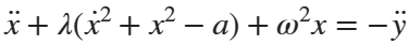
Setting the parameters (lambda = 3, a = 1, omega = 0.8, initial condition x0 = [3 -1]) I can get the acceleration of the system using the following code:

 

 

 

%% Init
clear variables
close all
clc
%% Code
% define parameters
lambda = 3;                                                                 % damping coefficient
% f = 0.8;       % [hz]                                                     % Frequency
% w = 2*pi*f;    % ~ 5[rad/sec]                                             % natural frequency
w = 0.8;                                                                    % natural frequency
a = 1;                                                                      % nonlinearity parameter
y = @(t) 0;
m = 90;

% define equation
f = @(t,x) [x(2); -lambda*(x(2)^2 + x(1)^2 - a)*x(2) - w^2*x(1) + y(t)];

% initial conditions
x0 = [3;-1];

% time span
tspan = [0 100];

% solve using ode45
[t,x] = ode45(f, tspan, x0);

% compute acceleration
xpp = -lambda*(x(:,2).^2 + x(:,1).^2 - a).*x(:,2) - w^2.*x(:,1) + y(t);

% plot solution
figure;
plot(t, xpp(:,1), 'b', 'LineWidth', 1.5);
xlim([40 50])
xlabel('t');
ylabel('xpp');
title('Acceleration of a Van der Pol Oscillator');
grid on

<

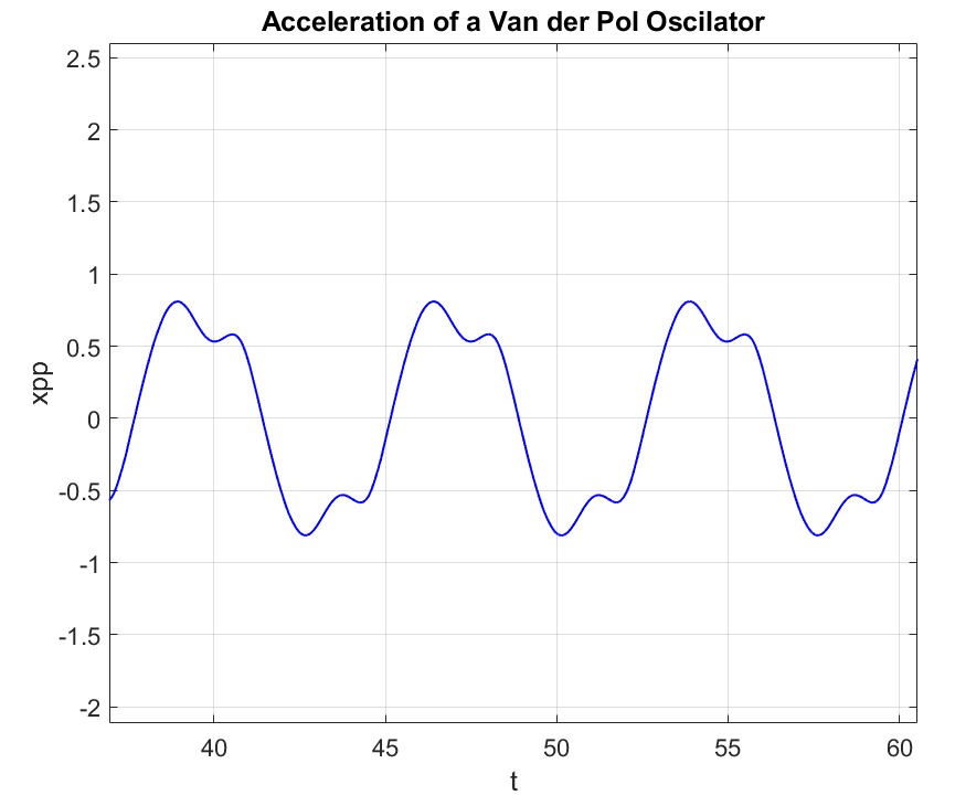
The shape looks like to the way a pedestrian applies lateral forces while walking according to multiple researches, BUT, the waves are far from each other. So my problem is that I want the waves come closer each other because the pedestrian frequency is approx f = 0.8[hz] or w = 2*pi*f = 5 [rad/sec] and as soon as I change the frequency the shape changes. I've been trying for hours to find a combination of parameters that produces exactly the same shape but the waves come closer to each other. Here is what I get (not the same shape, but I have the frequency)

Any help or recomendation to find the parameters?

 NOTE:-

Matlabsolutions.com provide latest MatLab Homework Help,MatLab Assignment Help , Finance Assignment Help for students, engineers and researchers in Multiple Branches like ECE, EEE, CSE, Mechanical, Civil with 100% output.Matlab Code for B.E, B.Tech,M.E,M.Tech, Ph.D. Scholars with 100% privacy guaranteed. Get MATLAB projects with source code for your learning and research.

Hi Alexis,

 

If you want to preserve the shape you will have to have a larger set of parameters. I am taking as given your equation

 

f = @(t,x) [x(2); -lambda*(x(2)^2 + x(1)^2 - a)*x(2) - w^2*x(1)]; (1)

where the y(t) term was taken away since it was set to 0 anyway. Rather than anonymous functions, there are two functions defined at the bottom of the script code below. The relevant line for the time derivatives is

dxy = [x(2); (-lam1*x(2)^2 -lam2*x(1)^2 +lam3*a)*x(2) - w^2*x(1)]

which is the same except there are three adjustable lambda values instead of just one. Suppose you start with (1) and want to speed up the waveform by a factor of b and change its size by a factor of A, all the while keeping the same shape. This can be done with

lam1 = lambda/(b*A^2);
lam2 = lambda*b/A^2;
lam3 = lambda*b;
and w --> w*b

If you speed up a waveform by a factor of b, then the acceleration goes up by a factor of b^2. The reason for A is that if you want to keep the acceleration the same as before, you can correct by a factor of A = 1/b^2. Or of course you can set the acceleration to any size, within reason.

The initial conditions should really be adjusted to get exact agreement for short times, but I left that alone because the solution settles down pretty quickly.

   SEE COMPLETE ANSWER CLICK THE LINK

https://www.matlabsolutions.com/resources/change-the-period-frequency-of-a-van-der-pol-oscillator.php