Noise samples of gaussian mixture distribution

 I'm new to matlab. I want to generate noise samples of Gaussian mixture with PDF= sqrt((u.^3)./pi).*exp(-u.*(x.^2)) + sqrt((1-u)^3/pi).*exp(-(1-u).*x.^2);

 

The length of noise sample is (1,200) Please help me out.

NOTE:-

Matlabsolutions.com provide latest MatLab Homework Help,MatLab Assignment Help for students, engineers and researchers in Multiple Branches like ECE, EEE, CSE, Mechanical, Civil with 100% output.Matlab Code for B.E, B.Tech,M.E,M.Tech, Ph.D. Scholars with 100% privacy guaranteed. Get MATLAB projects with source code for your learning and research.

Ok, so you have formulated what seems to me to be a rather strange mixture model.

 

You have two modes, with variances that are related to each other, the mean of both terms is zero.

 

So, if the PDF is:

 

PDF = sqrt((u.^3)./pi).*exp(-u.*(x.^2)) + sqrt((1-u)^3/pi).*exp(-(1-u).*x.^2)

So we have two terms there.

syms u positive
syms x real

Look at the first term:

pdf1 = sqrt((u.^3)./pi).*exp(-u.*(x.^2));
int(pdf1,x,[-inf,inf])
ans =
u

So, it integrates to u. The second term is similar,

pdf2 = sqrt(((1-u).^3)./pi).*exp(-(1-u).*(x.^2));
int(pdf2,x,[-inf,inf])
ans =
piecewise([u == 1, 0], [1 < u, Inf*1i], [u < 1, 1 - u])

For u <= 1, it integrates to 1-u.

 

So the integral of the sum is indeed 1, therefore it is a valid PDF.

 

Essentially, you have two Gaussian modes, such that the variances are 2/u and 2/(1-u) respectively. You have chosen the mixture parameter as the inverse of those variances. Effectively, when u is small (or very near 1), you have a mixture distribution that rarely, you will generate large outliers. When u is exactly 1/2, this reduces to a standard normal distribution, with a unit variance.

 

I'm not sure why, but I suppose that is not really important. Normally, one would choose a mixture parameter that is independent of the variances.

 

The solution is simple.

 

1. Pick some value for u. u determines both variances for each Gaussian mode, as well as the mixture coefficient.

2. For a sample size of N, pick N uniformly distributed random numbers. These will determine which mode you will sample from. Then just use a classical tool like randn to do the sampling.

 

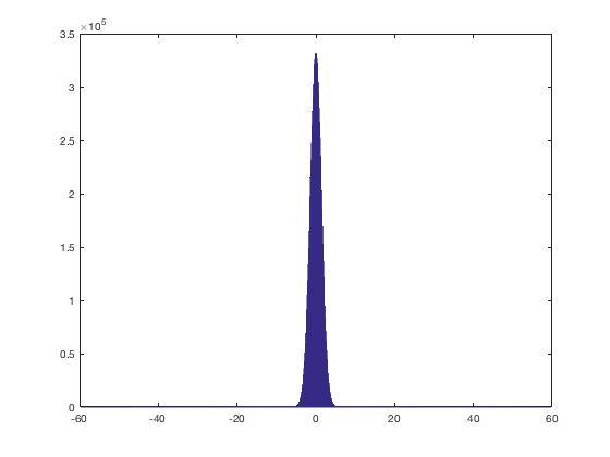
For a sample size of 1e7, and some arbitrary value for u, say 1/100. I've picked a tiny value for u to make the result clear. I've also chosen a large sample to make it easier to see as a histogram.

 

 

N = 10000000;
u = 0.01;

% random mixture selection
% Here s will be 1 if the element is sampled from first pdf.
%      s will be 0 if the element is sampled from second pdf.
s = rand(1,N) < u;

% sample using randn, with a unit variance initially
x = randn(1,N);;

% now scale each element based on the desired variance
x(s) = x(s)*sqrt(2/u);
x(~s) = x(~s)*sqrt(2/(1-u));

hist(x,1000)

So, for this fairly tiny value of u, see that the histogram looks much like a traditional Gaussian, BUT with very wide tails.

I'll next plot the separate pieces of the PDF, split into two parts. Here I've chosen u as 0.25.

 SEE COMPLETE ANSWER CLICK THE LINK

https://www.matlabsolutions.com/resources/noise-samples-of-gaussian-mixture-distribution.php